Prediction Model and Analyses

Author: Ivan Cano

Date: 3/8/2022

With the turn of the 21st century, the world has seen advancements in medicine, technology, and more equitable living standards in many parts of the world. And with this increase of human population, also comes expansion into human development, much of it in the form of housing and urban infrastructure. Although, in some cases, people may build settlements unsanctioned by the state, and these people may suffer many vulnerabilities, including increased crimes, and water and food insecurities in times of drought, natural disasters Our team believes that tracking human development can prove useful in helping these people that live on the fringes of society. By using satellite images, from the landsat 8 repository (a NASA satellite image database), our team has created labeling service to be able to classify urban settlement and expansion over periods of urban growth. In this markdown file we will be using information that we have gathered using our classification service on the Xiong An New District in Hebei, China to be able to accurately predict future growth by utiliying (machine learning) models. We hope that by creating an ml model to predict the urban expansion of this region in China we can prove the efectiveness of our labeling service and the accuracy of the service itself. Moreover, we will be analyzing the results found, to test if it aligns with general trends of the urban developement of the region to further test its our models accuracy. We hope that through the analyses we conduct in this project, we can promote people to use our service to aid communities. that live in rural areas across the world.

Data Cleaning​

import sklearn as sk
import numpy as np
import pandas as pd
import rasterio, os, napari
from sklearn.model_selection import train_test_split
from sklearn.ensemble import RandomForestClassifier
from sklearn.svm import SVC
from sklearn.cluster import KMeans
from sklearn.preprocessing import StandardScaler
from sklearn.datasets import load_iris
import functools

To begin, we conducted some data cleaning procedures with some replacement methods, removing any typos that could have occured in the labeling of urban and non_urban regions.

labels = pd.Series(labels).replace('non_urbn','non_urban').replace('non urban','non_urban').replace('Shapes','urban').replace('urban [1]', 'urban')
labels.value_counts()

labels = labels.replace('non_urban','temp')
labels = labels.replace('urban','temp_2')
labels = labels.replace('temp','urban')
labels = labels.replace('temp_2','non_urban') 

Training Random Forest Classifier​

Here we split the data with a training and a test set, with a 80% 20% split. This will allow us to train our model effectively, while still being able to test its performance.

 X_train, X_test, y_train, y_test = train_test_split(data,labels, test_size=0.2)

%matplotlib inline
import matplotlib.pyplot as plt
plt.style.use('seaborn-whitegrid')
import numpy as np

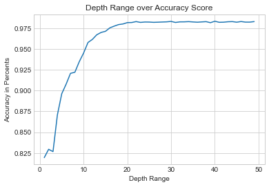
This is where we begin our hyperparameter optimization by testing a wide range of inputs and choosing the best performing input of the ones we tested. Much of the hyperparemeter tuning we performed here follows this logic, so for the sake of conciseness I won't be reitering this for the rest of the parameter tuning.

scores_depth = []
for i in range(1,50):
    fclf = RandomForestClassifier(max_depth=i, n_estimators=10, max_features=1)
    fclf.fit(X_train, y_train)
    scores_depth.append(fclf.score(X_test, y_test))

In this example it turned out the max depth was 25. In this example we added 1 to the location of the index of the highest score to compensate for the range we used starting at 1.

max_score = max(scores_estimators)
scores_estimators.index(max_score)
max_depth = scores_estimators.index(max_score)
max_depth += 1
max_depth

25

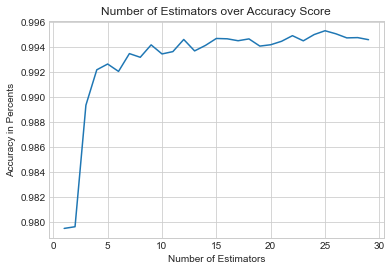
scores_estimators = []
for i in range(1,30):
    fclf = RandomForestClassifier(max_depth= max_depth, n_estimators=i, max_features=1)
    fclf.fit(data, labels)
    scores_estimators.append(fclf.score(data, labels))

plt.plot(range(1,30), scores_estimators)
plt.title("Number of Estimators over Accuracy Score")
plt.xlabel("Number of Estimators")
plt.ylabel("Accuracy in Percents");

max_score = max(scores_estimators)
max_estimators = scores_estimators.index(max_score)
max_estimators += 1
max_estimators

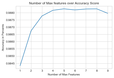
score_features = []
for i in range(1,10):
    fclf = RandomForestClassifier(max_depth = max_depth, n_estimators=max_estimators, max_features=i)
    fclf.fit(X_train, y_train)
    score_features.append(fclf.score(X_test, y_test))

plt.plot(range(1,10), score_features)
plt.title("Number of Max features over Accuracy Score")
plt.xlabel("Number of Max Features")
plt.ylabel("Accuracy in Percents");

max_score = max(score_features)
score_features.index(max_score)
max_features = score_features.index(max_score)
max_features += 1
max_features

5

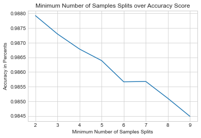
score_min_samples = []
for i in range(2,10):
    fclf = RandomForestClassifier(max_depth = max_depth, n_estimators=max_estimators, max_features=max_features, min_samples_leaf = i)
    fclf.fit(X_train, y_train)
    score_min_samples.append(fclf.score(X_test, y_test))

plt.plot(range(2,10), score_min_samples)
plt.title("Minimum Number of Samples Splits over Accuracy Score")
plt.xlabel("Minimum Number of Samples Splits")
plt.ylabel("Accuracy in Percents");

max_score = max(score_min_samples )
score_min_samples.index(max_score)
min_samples = score_min_samples.index(max_score)
min_samples += 2
min_samples

Here we test our values that we got from the hyperparameter optimization and fit them into our final rRandomForestClassifier. Theoreticaly this model should be well suited to classify regions based on urban and non_urban regions with with similar geographic properties as the Xiong An New District we used for our classifcation model.

Testing our model on the training dataset we can see that we scored a significantly high score of 98.7% accuracy. This definitily promising to applying our models on other regions of Hebei that are like Xiong An New District. That being said it should be mentioned that our model had not shown to perform significantly well in other datasets that do not share similar geographic properties. For example, as our first datasets includes many areas that are marsh like, from the large rice fields in Xiong An New District, it may not perform as well in other regions that have dry soil. Noteabley, for our second datset it was observed that our model perform significantly worse the region of Xushui District that do not share the same agricultural farmlands as the Xiong An New District. Therefore, our model should only be used in consideration of geographic regions that mimic the region we used as it may be prone to decreases in accuracy if used in ill suited regions.

fclf = RandomForestClassifier(max_depth = max_depth, n_estimators=max_estimators, max_features=max_features, min_samples_leaf = min_samples)
fclf.fit(X_train, y_train)
fclf.score(X_test, y_test)

0.987948551000602 ]

Analyses of Prediction Model​

Here we used our ml model we made in the previous step and processed the saved data we have in our testing_data/full_img/, already filled in the data_collection portion of this project. Although any tif files of the same dimensions as the images used for our train model could theoreticaly be used.

from os import listdir
from os.path import isfile, join

onlyfiles = [f for f in listdir(full_directory) if isfile(join(full_directory, f))]

model_predictions = []
for i in onlyfiles:
    with rasterio.open('testing_data/full_img/'  + i) as src:
    #     print(src.shape)
        img = src.read()
#     img.flatten(order = 'C')
    
        img_test = np.rollaxis(img.reshape(16,e_dims[1]*e_dims[2]),0,2)

        model_predictions.append(fclf.predict(img_test))

Here, we parse through the labels that we went acquired through our ml model. We then counted all the urban labels and and non_urban labels and created a ratio from these two value, where the length of urban labels was divided over the length of non_urban labels to get our desaired ratio.

urban_ratio = []
for i in model_predictions:
    urban_count = 0
    for j in i:
        if j == 'urban':
            urban_count += 1
#     print(urban_count)
    non_urban_count  = len(i) - urban_count
    urban_ratio.append(urban_count/non_urban_count)

import datetime

Here we pull all the names of the images we used for our ml model so that we could extract the dates associated with each tif file. We were able to extract the dates from the images by slicing their names which contained their associated dates and appended those dates to a list. We then formated and changed data type of the dates to datetime.date objects to better process the dates in our analyses.

onlyfiles[0][6:16]
dates = []
for i in onlyfiles:
    dates.append(i[6:16])

x_values = [datetime.datetime.strptime(d,"%Y-%m-%d").date() for d in dates]
x_values

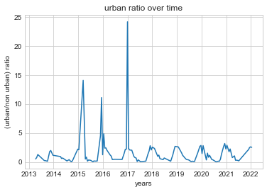
This graph represents the raw distribution of the data between the years April 10, 2013 to present day. Notable outliers can be observed here.

plt.plot(x_values, urban_ratio)

import numpy as np
import scipy.stats as st

The following lines are code to be able to be able to average out the urban ratios for every datapoint to be able to observe any discernable trend.

year_list = []
for i in x_values:
    year_list.append(i.year)

years = np.unique(year_list)

Here we initialize a dictionary to be able to classify the unique years in our datasets and set them as keys.

year_avg = {}
for i in years:
    year_avg[i] = []

We then fill these dictionaries with the values associated to every year.

pd.Series(year_list).value_counts()
for count, value in enumerate(urban_ratio):
    year_avg[year_list[count]].append(value)

Bellow we average out the data, and print out the output. Each value bellow is chronological where the first entry is the average of year 2013, and the last being the average of year 2022.

Unfortunrately because of some extreem outliers that could be seen earlier in our data, some years have, such as April have higher than average scores.

list_year_average = []
for i in year_avg:
    list_year_average.append(np.mean(year_avg[i]))
list_year_average

[0.8932386322805885, 0.5961964284060416, 2.541952400843471, 3.257714599207024, 1.249241606661275, 1.3375268946199286, 1.0263152629146564, 1.1877434043813473, 1.450091265543045, 2.5116910229645093]

To correct the discrepency in the data we decided to filter for any extreem outlier. As very few points scored higher than a 4, we decided to remove any outlier higher than this limit.

urban_ratio_corrected  = urban_ratio.copy()
bad_index = []
x_values_corrected = x_values.copy()
for i in urban_ratio_corrected:
   if i > 4:
       outlier_index = urban_ratio_corrected.index(i)
       bad_index.append(outlier_index)
count = 0
for i in bad_index:
   urban_ratio_corrected.pop(i - count)
   x_values_corrected.pop(i - count)
   count += 1

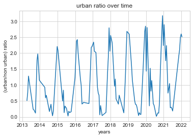
After removing any significant outliers the data took a form easier to interpret. The characteristics of the data seem to be ociliating respective to the beginings and ends of years. Additionaly there does seem to be a gradual increase to our urban score. It doesn't seem very drastic but it does seem present.

plt.plot(x_values_corrected, urban_ratio_corrected)
plt.title('urban ratio over time')
plt.xlabel('years')
plt.ylabel('(urban/non urban) ratio')
plt.show()

Converting dates to days​

TO further progress with the analyses of the data it was necessary to convert the values we have in our datetime.date objects to that of integers to be able to better process the data, and to test for further relationships it could have.

import datetime

Bellow we converted all the datetime.date objects to datetime.datetime using the timestop method in datetime.

my_date = x_values_corrected[0]
x_datetime = [datetime.datetime(i.year, i.month, i.day).timestamp() for i in x_values_corrected]

Once we had converted our object type to a datetime.datetime we then processed the tie in seconds to then be represented to time in minutes.

x_datetime_start = min(x_datetime)
x_datetime_days = [(x - x_datetime_start)/(60 * 60 * 24) for x in x_datetime]

Testing for Positive Trends​

x_minutes_reshaped = np.array(x_datetime_days).reshape((-1, 1))

Bellow we inputed our values into a linear regression model to see if our urban scores had any positive relationship over time. Analyzing our resulst we can see that there did seem to be positive coefficient of determination of 0.055, and a daily coefficient increase of 0.000236. COnverting the days into years yields a coefficient of a 0.086 increase of urban/non urban growth over a year. This certainly does seem to bode well for our classifcation service as an increase to urban/non urban growth indicates a growth in ubranization, as it should be considering that the Xiong An New District, the area from where our data is from is a new growing, and developing region in China that is suspected to have these kinda of growth.

import numpy as np
from sklearn.linear_model import LinearRegression
reg = LinearRegression().fit(x_minutes_reshaped, urban_ratio_corrected)
reg.score(x_minutes_reshaped, urban_ratio_corrected

0.05540008335192936

reg.intercept_

0.7142641939421813

reg.coef_

array([0.000236])

reg.coef_ * 365

array([0.08614175])

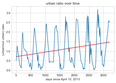
To visualized the relationship the linear relationship that our urban score has over time we displayed our information through a line graph. As our coeficients entailed, a positive coorelation can be observed to be illustrated in our graph through the red line. As iterated prior, this trend in the data indicating an increase in (urban labels/non urban labels) as time in days pass by (beginning from April 10, 2013) is indicative of urban expansion over time.

plt.plot(x_datetime_days, linear_relationship, label = "line 1", color = 'red')
plt.plot(x_datetime_days, urban_ratio_corrected)
plt.title('urban ratio over time')
plt.xlabel('days since April 10, 2013')
plt.ylabel('(urban/non urban) ratio')
plt.show()

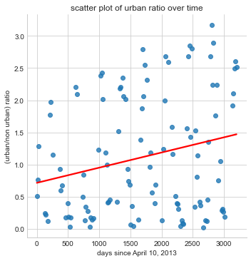
The following image is just a reiteration of our previouse data visualized but under a scater plot to observe the data under a different visual output.

!conda install --yes seaborn

x_series = pd.Series(x_datetime_days, name = 'x_datetime_days')
y_series = pd.Series(urban_ratio_corrected, name = 'urban_ratio_corrected')
df = pd.concat([x_series, y_series], axis=1)

import seaborn as sns

sns.lmplot(x='x_datetime_days', y='urban_ratio_corrected', data = df, fit_reg=True, ci=0, n_boot=1000, line_kws={'color': 'red'})
plt.title('scatter plot of urban ratio over time')
plt.xlabel('days since April 10, 2013')
plt.ylabel('(urban/non urban) ratio')
plt.show()

To adress some of the concerns we had about the ocilation in the data we decided to test for seasonality in the data as there seemed to be a pattern of regular patterns in increases and decreases in the urban scores in the data. It was suspected that this ocilation could be linked to different tempeture and weathers that change depending on the seasons of the year. This would make sense as our use in the NDSI band to label our image was intended to be used diferenciate between vegetation and urban areas in our data. Therefore it would also be logical to conclude that much of our labels of non_urban areas would also be highly dense in vegetation as that would be the regions in our labeling service that were most visualy diferentiable and would thus have been classified as non_urban. As such, our non_urban label variable would be highly susceptible to seasonal changes such in weather, especialy tempeture.

To test for this theory we went ahead and detrended the data to see if we could observe any notable changes in pattern to the graph.

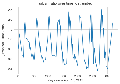
After detrending the data bellow, by removing any linear relationship between our two variables we plotted our data to test for seasonality. It can be observed that the data continuose to have a regular ocilating pattern that have regular intervals of increasing urban scores and decreasing urban scores, signifying possible trends to seasonality.

deseasonlized = (urban_ratio_corrected - linear_relationship) + reg.intercept_
plt.plot(x_datetime_days, deseasonlized)
plt.title('urban ratio over time: detrended')
plt.xlabel('days since April 10, 2013')
plt.ylabel('(urban/non urban) ratio')
plt.show()

Although to make sure that our prediction that our data included seasonal trends, we wanted to average out the data to see if we would still have that ocilation pattern that we have been observing thus far.

The processes to accomplish this was were simply to seperate all the dates to the months they pertained with, and to then average out their urban scores within datapoints of the same month.

month_list = []
for i in x_values:
    month_list.append(i.month)
months = np.unique(month_list)

Here is where parsed through the months and saved their urban score.

months_avg_corrected = {}
# year_avg.keys = years
for i in months:
    months_avg_corrected[i] = []
months_avg_corrected

months_list_corrected = []
for i in x_values_corrected:
    months_list_corrected.append(i.month)
len(months_list_corrected)

for count, value in enumerate(urban_ratio_corrected):
    months_avg_corrected[months_list_corrected[count]].append(value)

months_avg_corrected_2 = {}
for i in months_avg_corrected:
    months_avg_corrected_2[i] = np.mean(months_avg_corrected[i])

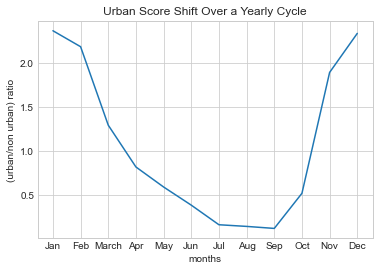
After averaging the data by months it can be observed that the urban score decreases as it aproaches the hoter dates in Hebei (May 10 to September 19), the province which our region is located in, and increases as it aproaches the colder dates (November 25 to February 24).

month_names = ['Jan', 'Feb', 'March', 'Apr', 'May', 'Jun', 'Jul', 'Aug', 'Sep', 'Oct', 'Nov', 'Dec']
year_avg_corrected = plt.plot(month_names,months_avg_corrected_2.values())
plt.title('Urban Score Shift Over a Yearly Cycle')
plt.xlabel('months')
plt.ylabel('(urban/non urban) ratio')
plt.show()

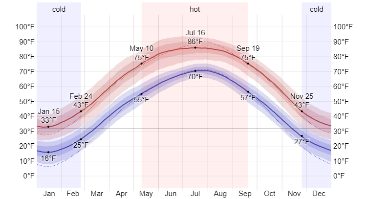
Furthermore, meterological trends back up our findings.weatherspark, a weather related database has very similar graphical representations that align with our studies. Unfortunately our team does not have access to this data to compare our statistical findings to their. And because of the time constraint of our project we were unable to do further research into seasonality. So we can only reference visual representation as that is what time and resources permits in our project.

In summary, through the random forest classifier it was found that urban expansion seemed to take place between the years 2013 and 2022 in the Xiong An New District we gathered from the banded data collected in the data processing portion of our project. We were able to accomplish analyzing this trend by creating a scoring system using based on a frequency of urban to non urban ratio we gathered after classifying our data into these two cattegories. Once we processed the data and extracted the dates for these urban scores, we were able to graph the progression of the data over time, which revealed to have a positive coefficient of 0.055. These results can be interpreted as there being an increase of urban expansion over time as the urban score of urban labels/non_urban labels increased over time. Additionaly it was found out that, some additional trends such as the oscillation in the data distribution could be attributed to seasonal changes. Fortunately this oscilation did not affect the results of our finding in relation to our models positive coorelation between time and urban expansion.